Descending networks transform command signals into population motor control

Fly stocks and husbandry

All experiments were performed on female adult D. melanogaster raised at 25 °C and 50% humidity on a 12-h light–dark cycle. The day before optogenetic experiments (22–26 h prior), we transferred experimental and control⁶¹ flies to a vial containing food covered with 20 μl all trans-retinal (ATR) solution (100 mM ATR in 100% ethanol; Sigma Aldrich R2500, Merck) and wrapped in aluminium foil.

Functional imaging and behaviour experiments

We generated transgenic flies expressing LexAop-opGCaMP6s (a gift from O. Akin⁶²) under the control of a Dfd-LexA driver (a gift from J. Simpson⁶³) and having a copy of UAS-CsChrimson (Bloomington ID 55135) (Supplementary Table 1, ID 1). We also generated flies that additionally had the LexAop-tdTomato transgene (Bloomington ID 77139) (Supplementary Table 1, ID 2). For most experiments, we used flies without tdTomato expression.

MDN-spGAL4 flies (also known as MDN3 from ref. ²) were used to drive backwards walking. aDN2-spGAL4 flies (also known as aDN2-spGAL4-2 from ref. ⁴) were used to drive antennal grooming. DNp09-spGAL4 flies (from ref. ³) were used to drive forwards walking. Their genotypes^{2,3,4,14,15,22,64} are listed at the top of Supplementary Table 2.

For all experiments in Figs. 2 and 4, we crossed spGAL4 flies or wild-type flies (Phinney Ridge flies, Dickinson laboratory) with one of our stable transgenic driver lines for imaging (Supplementary Table 1, ID 1 or ID 2). For Fig. 2, flies were 2–9 days post-eclosion and experiments were performed at Zeitgeber time 7–13 (ZT7–13). For Fig. 4, flies were 2–9 days post-eclosion and experiments were performed at ZT4–7. For Fig. 5, Extended Data Figs. 5, 6 and 10, we crossed spGAL4 lines with 20XUAS-CsChrimson.mVenus (attP40) flies (Bloomington ID 55135). Control experiments were performed by crossing wild-type flies (Phinney Ridge flies, or Canton S) to 20XUAS-CsChrimson.mVenus (attP40). The exact genotypes of the split lines and the source stocks are listed in Supplementary Table 2. All experiments were performed on flies 4–8 days post-eclosion at ZT4–7.

Confocal imaging experiments

We generated flies with stable Dfd-driven expression of membrane-targeted tdTomato or nuclear-targeted mCherry based on flies generated by the McCabe laboratory (EPFL) (Supplementary Table 1, IDs 3 and 4). For the three spGAL4 driver lines targeting comDNs (MDN, DNp09 and aDN2), we generated stable lines expressing CsChrimson (Supplementary Table 1, IDs 5, 6 and 7). We crossed flies expressing a red fluorescent protein variant with flies expressing CsChrimson in a spGAL4 driver line to visualize the expression patterns using confocal microscopy (Extended Data Fig. 1).

Recording from DNs using a Dfd driver line

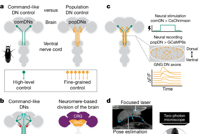
We leveraged a genetic-optical intersectional approach to selectively record from GNG DNs. We chose to record from GNG DNs because we found that 73% of all DN–DN synapses in the brain connectome are in the GNG. In addition, the GNG houses 60% of all DNs and 85% of all DNs have axonal output in the GNG¹⁴. However, the Hox gene Dfd does not include the entirety of all GNG DNs: it excludes those driven by the Hox gene Sex combs reduced (Scr)⁶⁵. Sterne et al.¹⁵ have estimated that 550 cells in the GNG are Dfd positive and 1,100 are Scr positive, with only a small fraction expressing both. We show, for example, that aDN2, although localized to the GNG, is Dfd negative and thus most likely Scr positive (Extended Data Fig. 1c). In our study, functional imaging of DNs using an Scr driver line proved difficult because Scr expression extends into the neck and anterior VNC⁶³. Specifically, we observed strong expression of GCaMP in the tissues surrounding the thoracic cervical connective (potentially ensheathing glia⁶⁶), making it very hard to record the activity of DN axons. We expect that some Scr-positive DNs will also be recruited by comDNs. Thus, we probably under-report the number of recruited GNG DNs.

Limitations of selected spGAL4 driver lines

In addition to descending neurons, our aDN2-spGAL4 driver line (aDN2-GAL4.2 (ref. ⁴)) contains two more groups of neurons. One pair is on the anterior surface of the brain and, based on our control experiments, is probably not or only weakly activated by targeted optical stimulation of the neck (and not at all activated by thoracic stimulation). Another is a set of neurons in the anterior VNC. Because other driver lines targeting aDN2 neurons with more, different off-target neurons have the same behavioural phenotype as our aDN2 driver⁴, we are confident that the effects that we observed are due to stimulating aDN2 neurons.

Different studies have reported variable behavioural phenotypes for stimulating the DNp09-spGAL4 driver line: some saw forwards walking³, whereas others observed stopping or freezing^18,67. We observed both: at our standard 21-μW optogenetic stimulation power, heterozygous animals mostly walked forwards. Occasionally, flies would only transiently walk forwards and then stop, or alternate rhythmically between walking and stopping. With higher expression levels of CsChrimson (that is, DNp09-spGAL4 > UAS-CsChrimson homozygous animals), we observed mostly freezing. We used heterozygous animals for our study.

Immunofluorescence tissue staining and confocal imaging

We dissected brains and VNCs from 3 to 6 days post-eclosion female flies as described in ref. ⁶⁸.

For samples in Extended Data Fig. 1a,c, we fixed flies in 4% paraformaldehyde (PFA; 441244-1KG, Sigma Aldrich, Merck) in 0.1 M PBS (Gibco PBS, pH 7.4, 10010-015, Thermo Fisher Scientific). We then washed them six times for 10 min with 1% Triton (Triton X-100, X100-100ML, Sigma Aldrich, Merck) in PBS (hereafter named 1% PBST) at room temperature. We then transferred them to a solution of 1% PBST, 5% natural goat serum (goat serum from controlled donor herd, G6767-100ML, Sigma Aldrich, Merck) and primary antibodies (see Supplementary Table 3) and left them overnight at 4 °C. We then washed the samples six times for 10 min with 1% PBST at room temperature. We transferred them to a solution of 1% PBST, 5% natural goat serum and secondary antibodies (see Supplementary Table 3) and left them for 2 h at room temperature. We then washed the samples six times for 10 min with 1% PBST at room temperature. We mounted the samples on glass slides using SlowFade (SlowFade Gold Antifade Mountant, S36936, Thermo Fisher Scientific) and applied a coverslip. To space the slide and the coverslip, we placed a small square of two layers of double-sided tape at each edge. We sealed the edges of the coverslip with nail polish.

For samples in Extended Data Fig. 1b, we fixed flies in 4% PFA in PBS and transferred them to 1% PBST and left them overnight at 4 °C. We then washed the samples three times for 15 min with 1% PBST at room temperature. We transferred them to a solution of 1% PBST, 5% natural goat serum and primary antibodies (see Supplementary Table 3) and left them overnight at 4 °C. We then washed the samples three times for 15 min with 1% PBST at room temperature. We transferred them to a solution of 1% PBST, 5% natural goat serum and secondary antibodies (see Supplementary Table 3) and left them overnight at 4 °C. We then washed the samples three times for 15 min with 1% PBST at room temperature. We mounted the samples on glass slides using SlowFade and applied a coverslip. To space the slide and the coverslip, we applied a small square of two layers of double-sided tape at each edge. We sealed the edges of the coverslip with nail polish.

We imaged samples using a Leica SP8 Point Scanning Confocal Microscope with the following settings: ×20, 0.75 NA HC PL APO dry objective, 2× image averaging, 1,024 × 1,024 pixels, 0.52 × 0.52-μm pixel size, 0.5-μm z-step interval; green channel 488-nm excitation, 50–540-nm emission bandpass; red channel (imaged separately to avoid cross-contamination) 552-nm excitation, 570–610-nm emission bandpass; and infrared channel (nc82, imaged in parallel with the green channel) 638-nm excitation, 650–700-nm emission bandpass. We summed confocal image stacks along the z-axis and rotated and translated the images to centre the brain/VNC using Fiji⁶⁹.

Optogenetic stimulation system and approach

We used a 640-nm laser (Coherent OBIS 1185055 640 nm LX 100 mW, Edmund Optics) as an optogenetic excitation light source. We reduced the light intensity using neutral density filters (Thorlabs) and controlled the light intensity with mixed analogue and digital control signals coming from an Arduino with custom software. A digital signal was used to turn the laser on and off. An analogue signal (PWM output from Arduino and RC low-pass filtered) was used to modulate the power. Both of those signals were sent in parallel to the laser and acquisition board and were recorded alongside the two-photon microscope signals using ThorSync 3.2 software (Thorlabs). The light was directed towards the fly with multiple mirrors. Fine control of the target location was achieved using a kinematic mount (KM100, Thorlabs) and a galvanometric mirror (GVS011/M, Thorlabs). We manually optimized targeting of the laser onto the neck/thorax before each experiment. The light was focused onto the fly using a plano-convex lens with f = 75.0 mm (LA1608, Thorlabs) placed at the focal distance from the fly. For stimulation of the inhibitory opsin GtACR1, we used the same system, but with a 561-nm laser (Coherent OBIS 1280720 561 nm LS 150 mW, Edmund Optics) instead of a 640-nm laser to better match the optical excitation spectrum of GtACR1.

We note that, although comDNs have axon collaterals in the GNG, none of the comDNs in this study were among the DN populations that we imaged: DNp09-spGAL4 and MDN-spGAL4 lines drive expression in neurons with cell bodies in the cerebral ganglia and not in the GNG (Extended Data Fig. 1a). The DN cell bodies of the aDN2-spGAL4 line are within the GNG but do not overlap with Dfd driver line expression (Extended Data Fig. 1c). Thus, we could be certain that any active DNs would be recruited through synaptic connections and not optogenetically. We identified laser light intensities that could elicit robust forwards walking, anterior grooming and backwards walking (Fig. 2a and Extended Data Fig. 1d).

We used different laser intensities to stimulate MDN (21 μW), DNp09 (21 μW) and aDN2 (41.6 μW) animals because 21-μW stimulation power mostly causes aDN2 animals to stop (Extended Data Fig. 1d). Activation of MDN in the head, neck and thorax was sufficient to trigger backwards walking (Extended Data Fig. 1e). Although some tissue scattering of laser light can be expected, in control experiments, we found that activation of the head capsule, but not the thorax, could strongly elicit forwards walking in the ‘bolt protocerebral neurons’ of the brain—these neurons are known to drive robust and fast forwards walking³ (Extended Data Fig. 1f). Stimulation (21 μW) was more specific than 41.6 μW, which is why we selected 21-μW stimulation for MDN and DNp09 as well as the spGAL4 lines tested (Fig. 5f,g and Extended Data Figs. 5 and 6). We regularly calibrated the laser intensity by measuring it with a power metre (PM100D, Thorlabs) and adjusting the analogue gain of the laser.

In vivo two-photon calcium imaging experiments

We performed two-photon microscopy with a ThorLabs Bergamo II two-photon microscope augmented with a behavioural tracking system as described in ref. ²⁹. In brief, we recorded a coronal section of the thoracic cervical connective using galvo-resonance scanning at around 16-Hz frame rate. In addition, optogentic stimulation was performed as described above. We only recorded the green PMT channel (525 ± 25 nm) because the red PMT channel would be saturated by red laser illumination of the fly. In parallel, we recorded animal behaviour at 100 frames per second (fps) using two infrared cameras placed in front and to the right of the fly.

Flies were dissected to obtain optical access to the VNC and thoracic cervical connective as described in ref. ⁷⁰. In brief, we mounted the fly to a custom stage by gluing its thorax and anterior head to the holder and removed its wings. Then, we opened the dorsal thorax using a syringe needle and waited for indirect flight muscles to degrade for approximately 1.5 h. We pushed aside the trachea and resected the gut and salivary glands. For some flies, where the trachea was obstructing the view, we placed a V-shaped implant⁷¹ into the thoracic cavity to push the trachea aside. We then placed the fly over an air-suspended spherical treadmill marked with a pattern visible on infrared cameras for ball tracking (air flow at 0.6 l min⁻¹). While the fly was adapting to this new environment (approximately 15 min), the imaging region was identified and the optogenetic stimulation laser was centred onto the neck.

We used ThorImage 3.2 to record and ThorSync 3.2 software to synchronize imaging data. We recorded 10,000 microscopy frames (around 10 min) while also recording behavioural data using cameras placed around the fly and presenting optogenetic stimuli. During a typical 10-min recording session, we presented 40 stimuli (5-s stimulation and 10-s inter-stimulus intervals). Whenever the recording quality was still good enough (that is, many neurons were visible and the fly still behaved healthily), we recorded multiple sessions to increase the number of stimulation trials. Many GNG DNs were active during spontaneous behaviour in the absence of optogenetic stimulation. Thus, to distinguish between GNG DN activity due to comDN stimulation versus the spontaneous initiation of behaviours, we only analysed trials for which flies were walking immediately before optogenetic stimulation. Because flies were quite spontaneously active, analysing trials for which flies were previously walking instead of resting increased the data available for trial averaging. It also allowed us to avoid laser light causing quiescent control animals to behave, obscuring our analyses.

Investigating natural behaviours

In Extended Data Fig. 2, we compared optogenetically elicited neural activity to activity observed during natural behaviours: forwards walking, anterior grooming and backwards walking. Natural forwards walking is frequently spontaneously generated by the flies. By contrast, we needed to stimulate the antennae with 5-s puffs of humidified air to increase the probability of natural grooming (Extended Data Fig. 2b). We provided humidified air puffs with an olfactometer (220A, Aurora Scientific) using the following parameters: 80 ml min⁻¹ air flow, 100% humidity, 5-s duration and 20-s inter-stimulus interval. To have humid air puffs (that is, an abrupt change in flow rate) instead of a switch from dry air to humidified air—the default olfactometer configuration—we only connected the ‘odour’ tube to the final valve and not the ‘air’ tube. Furthermore, to increase the likelihood of spontaneous backwards walking (Extended Data Fig. 2c), we replaced the spherical treadmill with a custom cylindrical treadmill that we found increases the motivation to backwards walk. Specifically, we designed a 10-mm diameter, 80-mg 3D-printed wheel (RCP-30 resin) and printed it using stereolithography through digital light processing (Envisiontec Perfactory P4 Mini XL). This wheel was mounted on a low-friction jewel-bearing holder (ST-3D sapphire shafts, VS-40 sapphire bearings, Freudiger SA). We marked the sides of the wheel with infrared-visible dots to facilitate infrared camera tracking of rotations and calculations of velocity to classify bouts of backwards walking. When using the wheel, we added an additional third infrared camera to the left of the wheel, where dot markers were visible.

Recording neuronal activity of DNs after resecting the VNC

To record neuronal activity in Dfd DNs after cutting the VNC, we first mounted and dissected flies as described above for intact animals. We verified that the animal was responding to optogenetic stimulation where appropriate and that the animal was still healthy. Then, we used a pair of microscissors (FST, Clipper Neuro Scissors, no. 15300-00, Fine Science Tools GmbH) to cut the entire VNC in the T1 neuromere. We cut just posterior to the fat bodies surrounding the cervical connective. We verified that the VNC was cut by pulling on its posterior region with forceps. We then performed two-photon imaging and optogenetic stimulation as in experiments with intact flies (that is, laser stimulation of the neck while recording a cross-section of the cervical connective). We recorded 5,000 microscopy frames (around 5 min) with 20 stimulation repetitions. Flies were hanging freely from the stage and not placed on the spherical treadmill because the VNC was injured resulting in no notable leg movements. Post-hoc, we recorded a volume stack of the cervical connective and T1 neuromeres to verify the location of the cut.

Behavioural experiments in leg-amputated animals

To investigate the number of actively controlled appendages involved in forwards and backwards walking, we mounted flies to the same stages used for imaging and behaviour experiments. We recorded ten trials of responses to optogenetic stimulation on the spherical treadmill, leaving 25 s between each stimulation. We then used cold anaesthesia to amputate the legs of the flies, before letting the flies recover for at least 10 min. The amputation was performed bilaterally for either the front legs, mid-legs or hindlegs, using clipper scissors (FST, Clipper Neuro Scissors, no. 15300-00, Fine Science Tools GmbH). We amputated the legs at the level of the tibia–tarsus joint to minimize the lesion while removing tarsal adhesion. Once they recovered, we recorded flies again on the spherical treadmill for ten trials. The control flies used to investigate walking phenotypes were Canton S, in accordance with previous work on locomotion—in particular DNp09 (ref. ³).

Behavioural experiments in headless animals

For behavioural experiments, we mounted flies to the same stages used for two-photon imaging, but without gluing the anterior part of the head to the holder. Then, without further dissection, we placed animals onto the spherical treadmill. After recording ten trials of responses to optogenetic stimulation in intact animals, we decapitated the fly by inverting the holder and pushing a razor blade onto the neck. To achieve this, we mounted a splinter of the razor blade onto the tip of a pair of dissection forceps for finer control. We took care not to injure the legs of the fly and to make a clean cut without pulling out thoracic organs passing through the neck connective. To limit desiccation, we then sealed the stump of the neck with a drop of UV-curable glue. We only continued experiments on flies if their limbs were moving following decapitation. We then placed the headless flies onto the spherical treadmill and let them recover for at least 10 min. Then, we recorded ten trials of responses to optogenetic stimulation on the spherical treadmill and ten trials in which the fly was hanging from the holder without contacting the spherical treadmill. In experiments for testing connectome-based predictions, we slightly modified this experimental procedure. Because intact control animals become aroused by optogenetic stimulation, to avoid false positives and to discover behavioural phenotypes for less well-studied DNs, we attempted to reduce the spontaneous movements of flies. First, instead of 10 s between optogenetic stimulation trials, we used 25 s. Second, we filled the fly holder with room temperature saline solution to buffer heating from infrared illumination. For Extended Data Figs. 5 and 6, control flies (no DN > CsChrimson) were of the Phinney Ridge genetic background except for the later-studied DNp42, oviDN and DNg11, which were compared with control flies of the Canton S genetic background.

Data exclusion

We manually scored the quality of neural recordings (signal-to-noise ratio, occlusions, and so on) and the behaviour of the fly (rigidity, leg injury, among others) on a scale from 1 to 6 (where 1 is very good, 3 is satisfying and 6 is insufficient) for each 10-min recording session. We only retained sessions in which both criteria were at least at a ‘satisfying’ quality level. Unless indicated otherwise, we analysed trials in which the fly was walking before stimulus onset. Thus, we did not retain data from flies with less than ten trials of walking before stimulation. We chose to do this for several reasons: (1) GCaMP6s decays very slowly. Even if the fly was moving approximately 2 s before stimulation, we still observed residual fluorescence signals, increasing the variability of changes upon stimulation. There were only very few instances in which the animal was robustly resting for more than 2 s, making the inverse analysis impossible. (2) We observed that control flies became aroused upon laser light stimulation. Thus, they may begin moving if they were resting before stimulation, indirectly driving DN activity and making it harder to discriminate between optogenetically induced versus arousal-induced activity. Data from flies that were resting before stimulation exhibit recruitment patterns that are similar, although not identical (see data at https://doi.org/10.7910/DVN/HNGVGA). DNp09 shows strong activation in the medial cervical connective (as for when the fly was walking before stimulation) and additional activation in lateral regions. The central neurons characteristic of aDN2 activation in animals that were previously walking are also active in animals that were previously resting. In addition, we observed more widespread, weaker activation. DN signals upon MDN activation were slightly more spread out when the fly was resting before stimulation.

For experiments with headless animals, we excluded data from flies in which one of the legs was visibly immobile after decapitation, when at least one leg was not displaying spontaneous coordinated movements, or when the abdomen was stuck to the spherical treadmill such that other movements became impossible.

Behavioural data analysis

For analysis, we used a custom Python code unless otherwise indicated. Code for behavioural data preprocessing can be found in the ‘twoppp’ Python package on GitHub (https://github.com/NeLy-EPFL/twoppp) previously used in ref. ⁷¹. Code for more detailed analysis can be found in the GitHub repository (https://github.com/NeLy-EPFL/dn_networks) for this paper.

Velocity computation

As a proxy for walking velocities, we tracked rotations of the spherical treadmill using Fictrac⁷². Data from an infrared camera placed in front of the fly were used for these measurements as described in ref. ²⁹. Raw velocity traces acquired at 100 Hz were noisy and thus low-pass filtered with a median filter (width = 5 = 0.05 s) and a Gaussian filter (σ = 10 = 0.1 s).

The velocity of the cylindrical treadmill was computed as follows. First, the wheel was detected in a camera on the left side of the fly using Hough circle detection. For each frame, we extracted a line profile along the surface of the wheel showing the dot pattern painted on its side. We then compared this line profile to the line profile of the previous frame to determine the most likely rotational shift. We converted this shift to a difference in wheel angle and then transformed this into a linear velocity in millimetres per second to make it comparable to quantification of spherical treadmill rotations. This image processing was prone to high-frequency noise. Therefore, we filtered raw velocities with a Gaussian filter (σ = 20 = 0.2 s).

2D pose estimation

We tracked nine keypoints from a camera on the right side of the fly: anal plate, ovipositor, most posterior stripe, neck, front leg coxa, front leg femur tibia joint, front leg tibia–tarsus joint, mid-leg tibia–tarsus joint and hindleg tibia–tarsus joint (see Fig. 1d) using SLEAP (v1.3.0)⁷³.

Behaviour classification

We classified behaviours using an interpretable classifier based on heuristic thresholds on the walking velocity, limb motion energy and front leg height. For example, we classified forwards and backwards walking as having a forwards velocity of more than 1 mm s⁻¹ and − 1 mm s⁻¹ or less, respectively. All parameters are shown in Supplementary Table 4. If none of the conditions was fulfilled, we classified the behaviour as undefined.

Anterior grooming was composed of a logical ‘OR’ of two conditions: (1) the front leg was lifted up high, or (2) the front leg was moving with high motion energy. Front leg height was computed as the vertical distance between the front leg tibia–tarsus joint and the median position of the coxa. Pixel coordinates start from the top of the image. Thus, it is positive when the front leg is low (for example, during resting) and negative when the front leg is high (for example, during head grooming). Motion energy (ME) of the front legs, mid-legs and hindlegs was computed based on the movements of the respective tibia–tarsus joint as follows: \({\rm{ME}}=\sqrt{{(\Delta {x}_{t})}^{2}+{(\Delta {y}_{t})}^{2}}\), where Δx_t and Δy_t are the difference in x and y between two consecutive frames. We then computed the moving average of the motion energy within a 0.5-s (that is, 50 samples) window to focus on longer timescale changes in motion energy.

Two-photon microscopy image analysis

We used a custom Python code unless otherwise indicated. For all image analysis, the y axis is dorsal–ventral along the body of the fly, and the x axis is medial–lateral. Image and filter kernel sizes are specified as (y, x) in units of pixels. Code for two-photon data preprocessing can be found in the ‘twoppp’ Python package on GitHub (https://github.com/NeLy-EPFL/twoppp) previously used in ref. ⁷¹. Code for more detailed analysis can be found in the GitHub repository (https://github.com/NeLy-EPFL/dn_networks) for this paper.

Motion correction

Recordings from the thoracic cervical connective suffer from large inter-frame motion including large translations, as well as smaller, non-affine deformations. Contrary to motion-correction procedures used before for similar data⁷¹, here we made use of the high baseline fluorescence seen in Dfd > LexAop-GCaMP6s animals instead of relying on an additional, red colour channel for motion correction. Thus, we performed motion correction directly on the green GCaMP channel. We compared the performance for data where a red channel was available and could only find negligible differences in ROI signals. Whether a neuron was encoding walking or resting was unchanged irrespective of whether we used the GCaMP channel or recordings from an additional red fluorescent protein.

We performed centre-of-mass registration on every microscopy frame to compensate for large cervical connective translations. We cropped the microscopy images (from 480 × 736 to 320 × 736 pixels). Then, we computed the motion field for each frame relative to one selected frame per fly using optic flow. We corrected the frames for this motion using bi-linear interpolation. The algorithm for optic flow motion correction was previously described in ref. ⁷⁰. We only used the optic flow component to compute the motion fields and omitted the feature matching constraint. We regularized the gradient of the motion field to promote smoothness (λ = 800).

ROI detection

For each pixel, we computed the standard deviation image across time for the entire recording. This gives a good proxy of whether a pixel belongs to a neuron: it has high standard deviation because the neuron was sometimes active. We used this image as a spatial map of the recording to inform ROI detection. Example standard deviation images are also used as the background image for Fig. 2c.

We applied principal component analysis (PCA) on a subset of all pixels in the two-photon recording. We then projected the loadings of the first five principal components back into the image space. This gave us additional spatial maps integrating functional information to identify neurons. We then used a semi-automated procedure to detect ROIs; we performed peak detection in the standard deviation map. We visually inspected these peaks for correctness by looking at both the standard deviation map and the PCA maps. We manually added ROIs that the peak detection algorithm had missed, for example, because the neuron was only weakly active. The functional PCA maps allowed us to discriminate between nearby neurons with dissimilar functions. They might show up as one big peak in the standard deviation map, but would clearly be assigned to different principal components. We were able to annotate between 50 and 80 ROIs for each fly. The number of visible neurons varies due to GCaMP6s expression levels, dissection quality, recording quality and the behavioural activity level of the fly.

Neural signal processing

We extracted fluorescence values for each annotated ROI by averaging all pixels within a rhomboid shape placed symmetrically over the ROI centre (11 pixels high and 7 pixels wide). This gave us raw fluorescence traces across time for each neuron/ROI. We then low-pass filtered those raw fluorescence traces using a median filter (width = 3 = ~0.185 s) and a Gaussian filter (σ = 3 = ~0.185 s).

ΔF/F computation

Because of variable expression levels among cells, GCaMP fluorescence is usually reported as a change in fluorescence relative to a baseline fluorescence. Here we were mostly interested whether neurons were activated. To have a quantification that was comparable across neurons, we also normalized fluorescence of each neuron to its maximum level. Thus, we computed \(\Delta F/F=\frac{F-{F}_{0}}{{F}_{{{\max}}}-{F}_{0}}\), where F is the time-varying fluorescence of a neuron, F₀ is its fluorescence baseline and F_max is its maximum fluorescence. We computed F_max as the 95% quantile value of F across the entirety of the recording. In rare instances, neurons would get occluded, or slight glitches of the motion-correction algorithm would result in some residual movement. Both of these make it challenging to estimate the minimum fluorescence. When the fly is resting, nearly all neurons are at their lowest levels (aside from several²⁹) and there is usually less movement of the nervous system. Thus, we computed F₀ as a ‘resting baseline’ as follows. First, using our behavioural classifier, we identified the onset of prolonged resting (at least 75% of 1 s after onset classified as resting and at least 1 s after the previous onset of resting) outside of optogenetic stimulation periods. For each neuron, we then computed the median fluorescence across repetitions aligned to resting onset. We then searched for the minimum value in time over the 2 s following rest onset. Taking the median across multiple instances of resting provided a more stable way to compute the baseline than by simply taking the minimum fluorescence. For flies that were not behaving (that is, those with resected VNCs shown in Extended Data Fig. 3), we could not compute a resting baseline and instead used the 5% quantile value as F₀. The normalization using F₀ and F_max provided a way to compare fluorescence across multiple neurons with similar units. Thus, whenever we report absolute ΔF/F, a value of 0 refers to neural activity during resting and 1 refers to the 95% quantile of neural activity. When we report ΔF/F relative to pre-stimulus values (Fig. 2b–f,i and Extended Data Fig. 2), the unit of ΔF/F persists and a value of 0.5 means that the neuron has changed its activity level half as much as when it would go from a resting state to its 95% quantile state.

Video data processing

To process the raw fluorescence videos shown in Supplementary Videos 1 and 2 and in Fig. 2b, we first low-pass filtered the data with the same temporal filters as for ROI signals (median filter width = 3 = ~0.185 s, Gaussian filter σ = 3 = ~0.185 s). In addition, we applied spatial filters (median filter width = [3,3] pixels, Gaussian filter σ = [2,2] pixels). We then applied the same ΔF/F computation method described above, but for each individual pixel instead of for individual ROIs. Thus, the units used in the videos are identical to the units used for ROI signals in Fig. 2 and Extended Data Fig. 1.

Synchronization of two-photon imaging and camera data

We recorded two different data modalities at two different sampling frequencies: two-photon imaging data were recorded at approximately 16.23 Hz and behavioural images from cameras were acquired at 100 Hz. We synchronized these recordings using a trigger signal acquired at 30 kHz. When it was necessary to analyse neural and behavioural data at the same sampling rate (for example, Supplementary Videos 1 and 2), we downsampled all measurements to the two-photon imaging frame rate by averaging all behavioural samples acquired during one two-photon frame. In the figures, we report data at its original sampling rate.

Stimulus-triggered analysis of neural and behavioural data

We proceeded in the same way irrespective of whether the trigger was the onset of optogenetic stimulation (Figs. 2, 4 and 5 and Extended Data Figs. 1, 3, 5, 6 and 10) or the onset of a natural (spontaneous or puff elicited) behaviour (Extended Data Fig. 2). To compute stimulus-triggered averages, we aligned all trials to the onset of stimulation and considered the times between 5 s before the stimulus onset and 5 s after stimulus offset. In Fig. 2, we only considered trials in which the fly was walking in the 1 s before stimulation (behaviour classification applied to the mean of the 1-s pre-stimulus interval). We only considered flies with at least ten trials of walking before stimulation. Behavioural responses in Figs. 2a, 4b–g and 5f,g and Extended Data Fig. 1d–f, 2a–c, 5, 6 and 10 show the average across all trials (including multiple animals) and the shaded area indicates the 95% confidence interval of the mean across trials. When behavioural probabilities are shown, the fraction of trials that a certain behaviour occurs at a specific time after stimulus onset is shown. Neural responses over time in Fig. 2d and Extended Data Figs. 2a–c and 3c,h show average responses across all trials for one animal. To visualize the change in neural activity upon stimulation, the mean of neural activity in the 1 s before stimulation is subtracted for each neuron. If the absolute value of the mean across trials for a given neuron at a given time point was less than the 95% confidence interval of the mean, the data were masked with 0 (that is, it is white in the plot). This procedure allowed us to reject noisy neurons with no consistent response across trials. Because we subtracted the baseline activity before stimulus onset, we also observed DNs that became less active upon optogenetic stimulation (neurons appearing blue). However, GCaMP6s fluorescence does not reliably reflect neural inhibition. Thus, we cannot claim that this reduced activation in some neurons is due to inhibition. Instead, because the flies were walking before stimulation onset, those neurons most likely encode walking and became less active when the fly stopped walking forwards.

Individual neuron responses in Fig. 2c and Extended Data Fig. 2a–c,f and 3b,g show the maximum response of a single neuron/ROI. We detected the maximum response during the first half of the stimulus (2.5 s). We then computed the mean response of this neuron during 1 s centred around the time of its maximum response. If during at least half of that 1 s the mean was confidently different from 0 (that is, ∣mean∣ > CI), we considered the neuron to be responsive, otherwise we masked the response to zero to reject noisy neurons with no consistent response across trials. Figure 2b shows the same as Fig. 2c, but with this processing applied to pixels rather than individual neurons/ROIs. Contrary to previous ROI processing, pixels are not masked to 0 in case they are not responsive. Figure 2e shows an overlay of Fig. 2c for multiple flies. Data from each of these flies were registered to one another by aligning the y coordinates of the most dorsal and ventral neurons, as well as the x coordinate of the most lateral neurons. Figure 2f is a density visualization of Fig. 2e. To compute the density, we set the individual pixel values where a neuron was located to its response value and summed this across flies. We then applied a Gaussian filter (σ = 25 pixels, kernel normalized such that it has a value of 1 in the centre to keep the units interpretable) and divided by the number of flies to create an ‘average fly’. Extended Data Fig. 2d was generated in the same manner.

Statistical tests

Figure 2g–i includes a statistical analysis of neural responses. We quantified the number of activated neurons for each fly (Fig. 2g) as the neurons whose response value was positive (as in Fig. 2c). We quantified the fraction of activated neurons for each fly (Fig. 2h) by dividing the number of activated neurons by the number of neurons detected in the recording. In Fig. 2i, we quantified the summed ΔF/F as the sum of the response values of neurons that were positively activated (see the red line in Fig. 2d). Here we ignored neurons with negative response values because reductions in GCaMP fluorescence should not be interpreted as reflecting inhibition (see above). We used two-sided Mann–Whitney U-tests (scipy.stats.mannwhitneyu⁷⁴) to statistically analyse these comparisons. Sample sizes and P values are described in the figure legends. The Mann–Whitney U-test is a ranked test. Thus, comparing three samples against three samples (for example, aDN2 versus control), where all samples are at identical relative positions (that is, ranks), will yield the same P value, even if the absolute values are slightly different. This leads the P values to be identical across Fig. 2g–i, reflecting the conservative choice of a rank test that does not assume an underlying distribution.

Figures 4b–e and 5f,g and Extended Data Figs. 5 and 6 show statistical tests comparing the behavioural responses of intact and headless flies. Figures 4f,g and 5f,g and Extended Data Figs. 5 and 6 show statistical tests comparing the behavioural responses of headless experimental flies with headless control flies. In each case, we used two-sided Mann–Whitney U-tests (scipy.stats.mannwhitneyu⁷⁴) to compare the average value within the first 2.5 s after stimulus onset. We averaged across technical replicates (trials) and only compared biological replicates (individual flies) using statistical tests. Exact P values rounded to three digits are indicated in Supplementary Table 5.

Statistical tests in Extended Data Fig. 10 show comparison of the behavioural responses of leg-amputated experimental flies with intact experimental flies, and leg-amputated experimental flies with leg-amputated control flies. In each case, we used two-sided Mann–Whitney U-tests (scipy.stats.mannwhitneyu⁷⁴) to compare the total displacement after 5 s of stimulation. We averaged across technical replicates (trials) and only compared biological replicates (individual flies) using statistical tests. Exact P values rounded to three digits are in Supplementary Table 6.

Extended Data Fig. 2a–c (right) and 2e show the Pearson correlation between neural responses to optogenetic stimulation and neural activity during natural (spontaneous or puff-elicited) behaviours. The two-sided significance of the correlation is measured as the probability that a random sample has a correlation coefficient as high as the one reported (scipy.stats.pearsonr v1.4.1 (ref. ⁷⁴)).

In all figures showing statistical tests, significance levels are indicated as follows: ***P < 0.001, **P < 0.01, *P < 0.05 and not significant (NS) P ≥ 0.05.

Brain connectome analysis

Loading connectome data

We used the female adult fly brain (FAFB) connectomics dataset⁷ from Codex⁷⁵ (version hosted on Codex as of 3 August 2023, FlyWire materialization snapshot 630; https://codex.flywire.ai/api/download) to generate all figures. We merged the ‘neurons’, ‘morphology clusters’, ‘connectivity clusters’, ‘classification’, ‘cell stats’, ‘labels’, ‘connections’ and ‘connectivity tags’ tables. We then found DNs by filtering for the attribute super_class=descending. We identified DNs with known, named (for example, DNp09) genetic driver lines from Namiki et al.¹⁴ by checking the ‘cell type’, ‘hemibrain type’ and ‘community labels’ attributes (in this priority) and using the following rules. Otherwise, we used the consensus cell type³⁸ (for example, DNpe078). We semi-automatically assigned names using the following rules:

1. 1.

   For special neurons, we manually labelled root IDs 720575940610236514, 720575940640331472, 720575940631082808 and 720575940616026939 as MDNs based on community labels from S. Bidaye (consensus cell type DNpe078); root IDs 720575940616185531 and 720575940624319124 as aDN1 based on community labels from K. Eichler and S. Hampel (consensus cell type DNge197); and root IDs 720575940624220925 and 720575940629806974 as aDN2 based on community labels from K. Eichler and S. Hampel (consensus cell type DNge078). We verified visually that the shape of the neurons corresponded to published light-level microscopy images^2,4.

2. 2.

   Otherwise, if both the hemibrain_type attribute and the cell_type attribute followed the Namiki format (‘DN{1 lowercase letter} {2 digits}’, for example, ‘DNp16’) and they are identical, we used this as the cell name. If they are both in this format but are not identical, we marked this neuron for manual intervention.

3. 3.

   Otherwise, if the hemibrain_type attribute follows the Namiki format, we used this as the cell name. In addition, if the hemibrain_type attribute follows the Namiki format, but the cell_type attribute has a different value following the consensus cell-type format (‘DN{at least 1 lowercase letter} {at least 1 digit}’, such as ‘DNge198’), we marked the cell as requiring manual attention.

4. 4.

   Otherwise, if the cell_type attribute follows the Namiki format, we used this as the cell name.

5. 5.

   Otherwise, if the cell_type attribute follows the consensus cell-type format, we used this as the cell name.

6. 6.

   Otherwise, we marked the cell as requiring manual intervention.

7. 7.

   Wherever manual intervention was required (mostly in which the hemibrain_type is the Namiki format, but the cell_type is in the consensus cell-type format), we manually assigned the consensus cell type. However, we assigned the Namiki type if there was no other DN in this Namiki cell type or if the cell type was still missing a pair of DNs¹⁴.

Next, we stored the connectome as a graph using SciPy sparse matrix⁷⁴ and NetworkX DirectedGraph⁷⁶ representations. We identified DNs with somas in the GNG by checking the third letter of the consensus cell type to be ‘g’ (that is, DNgeXXX)³⁸.

Analysing connectivity

We only considered neurons with at least five synapses to be connected and computed the number of connected DNs based on this criterion (Figs. 3, 5b,c,e and 6a–c and Extended Data Figs. 4–9). This is the same value as the default in Codex, the connectome data explorer provided by the FlyWire community^37,75. Analysis of connectivity across three brain hemispheres (two brain halves from the FAFB dataset⁷ and one from the hemibrain dataset⁷⁷) revealed that connections “stronger than ten synapses or 1.1% of the target’s inputs have a greater than 90% change to be preserved”³⁸. We visualized all DNs connected to a given DN (Figs. 3a,b and 5d and Extended Data Figs. 5 and 6) using the neuromancer interface, and manually coloured neurons depending on whether they are in the GNG.

Neurotransmitter identification was available from the connectome dataset based on classification of individual synapses with an average accuracy of 87%³⁹. Here we report neurotransmitter identity for a given presynaptic–postsynaptic connection. To define neurotransmitter identity for a given presynaptic–postsynaptic pair, we asserted that the neurotransmitter type would be unique using a majority vote rule. This was chosen as a tradeoff between harmonizing neurotransmitters for a neuron (especially GABA, acetylcholine and glutamate⁷⁸) and avoiding the propagation of classification errors.

DN network visualizations and DN hierarchy

We used the networkx library⁷⁶ to plot networks of DNs in Figs. 3c,d and 5e and Extended Data Fig. 5–9. Again, we considered neurons to be connected if they had at least five synapses. In the circular plots, we show summed connectivity of multiple DNs. For example, the network for DNp09 in Fig. 3c shows only one green circle in the centre representing two DNp09 neurons. All connections shown as arrows are the sum of those two neurons. DNs are considered excitatory if they have the neurotransmitter acetylcholine and inhibitory if they have the neurotransmitter GABA. Whether glutamate is excitatory or inhibitory is unclear; this depends on the receptor subtype⁶⁰, which is unknown in most cases. To emphasize this, we highlight glutamatergic network edges in a different colour (pink).

In Fig. 3e, we show the cumulative distribution of the number of DNs reachable within up to n synapses. Statistics on DN connectivity across multiple synapses were computed using matrix multiplication with the numpy library on the adjacency matrix of the network. Lines in colour represent a DN network traversal starting at specific comDNs. The black trace represents the median of all neurons. Only a maximum of approximately 800 DNs can be reached because the others have maximally one DN input. In Fig. 5b,c, we sorted DNs by the number of monosynaptic connections that they make to other DNs. In Fig. 5b, the same sorting is applied to show the number of connected GNG DNs (orange).

In Extended Data Fig. 4, we show the effect of the choice of different constraints of the underlying connectome network on DN–DN connectivity degree. Statistics on DN connectivity across multiple synapses were computed using matrix multiplication with the numpy library on the adjacency matrices of the network. The segregation of excitatory and inhibitory connections was obtained by applying a mask on the direct connection signs. This implies that an inhibitory neuron acting on another inhibitory neuron would not be counted as excitatory but simply ignored in Extended Data Fig. 4d–f.

Fitting network models to connectivity degree distribution

In Fig. 6a, we generated a shuffled network of the same size by keeping the number of neurons constant and keeping the number of connections constant. Then, we randomly shuffled (that is, reassigned) those connections. Here we only considered the binary measure of whether a neuron was connected (number of synapses > 5) and not its synaptic weight. We then fit a power law or an exponential to the connectivity degree distribution using the scipy.optimize⁷⁴ library. Histograms of the degree distributions for all four distributions are shown in Fig. 6a using constant bin widths of five neurons. The quality of the fits are quantified using linear regression (R²).

Detection of DN clusters

We applied the Louvain method⁴⁸ with resolution parameter γ = 1 to detect clusters in the undirected network of DNs (that is, connections between two neurons are scaled by their synaptic strength and neurotransmitter identity, but the directionality of the connection is not taken into account). Here all connections—feedforward, lateral and feedback—are taken into account. In brief, the Louvain method is a greedy algorithm that maximizes modularity (that is, the relative density of connections within clusters compared with between clusters). To simplify analysing the network during the optimization, we did not consider the directionality of connections between neurons. If there is reciprocal connectivity between neurons, we add up the number of synapses (positive if excitatory, negative if inhibitory; here glutamate is considered inhibitory and neuromodulators are disregarded for the sake of simplicity). The Louvain method finds different local optima of cluster assignments due to its stochastic initialization and greedy nature. Therefore, we ran the algorithm 100 times. On the basis of the outcomes of these 100 runs, we defined a co-clustering matrix: the matrix has the same size as the connectivity matrix (number of DNs × number of DNs). Each entry represents how often two DNs end up in the same cluster. This matrix assigns each pair of DNs a probability to be in the same cluster. Using this meta-clustering, we could be sure that the sorting of DNs that we found through clustering is not a local optimum and that it is reproducible. We then applied hierarchical clustering to this matrix (using the ‘ward’ optimization method from the scipy.cluster.hierarchy library⁷⁴) to get the final sorting of DNs shown in Fig. 6b. We used this final sorting to detect the clusters shown in grey in Fig. 6b as follows: we started from one side of the sorted DNs and sequentially grew the cluster. If the next DN was in the same Louvain clusters at least 25% of the time, we assigned it to the same cluster as the previous DN. If not, we started a new cluster with this DN and kept testing subsequent DNs to determine whether they fulfil the criteria for this new cluster. Finally, we only kept clusters that had at least ten neurons. This yielded 12 clusters (grey squares). We applied this same meta-clustering and sorting approach to analyse the shuffled network (same number of DNs, same number of connections and same number of synapses, but shuffled connections). On this shuffled network, we found 34 clusters of much smaller size (Fig. 6c), hinting at a better clustering in our network than in a shuffled control (modularity = 0.27 for the original network and modularity = 0.12 for the shuffled network). The number of synapses is shown as positive (red) if it is excitatory and as negative (blue) if it is inhibitory.

We then analysed the connectivity within and between clusters. To do this, we accumulated the number of synapses between two clusters (positive for excitatory and negative for inhibitory). To be able to compare this quantity between clusters of different sizes, we divided this number of synapses by the number of DNs in the cluster that receives the synaptic connections. This quantity is visualized in Fig. 6d for the original DN–DN network clusters and Fig. 6e for the shuffled network as the ‘normalized number of synapses’. If positive (red), then connections from one cluster to another are predominantly excitatory. If negative (blue), then connections are predominantly inhibitory. We did not mirror connectome data before clustering because it requires resolving discrepancies between left and right neuron pairs, which, in many cases, are also not identifiable as corresponding cell classes across the brain.

Statistical comparison of original versus shuffled DN–DN clusters

As detailed above, we applied the Louvain algorithm 100 times to increase the robustness of clustering. We computed statistics on the clustering of this dataset (mean and standard deviation) specifically on metrics including the size and number of clusters. We then compared these distributions with those for the shuffled graph using one-sided Welch’s t-tests (scipy.stats.ttest_ind⁷⁴ with equal_var = False). The resulting statistics are a conservative quantification of the difference between the original network and the shuffled control, as each data point is taken independently. When performing the hierarchical clustering across 100 iterations, the large clusters from the biological network are preserved, whereas the random associations of the shuffled network become incoherent. In practice, the difference in cluster sizes reported statistically underestimates the difference between the resulting matrices shown in Fig. 6b,c. The 100 iterations result from random seed initialization, on the condition that the algorithm converges. We restarted it whenever the convergence criteria were not reached within 3 s. Indeed, we observed empirically that when the algorithm would not converge in 3 s, it would not do so for at least 30 min and was, therefore, terminated.

Identifying DNs to test predictions

On the basis of the cell-type data associated with each neuron in FAFB (see above), we were able to find many DNs from refs. ^{4,14,15,22,64} in the connectome database. We then checked which of them have either a very high number of synaptic connections to other DNs or a very low number. We then filtered for lines where a clean spGAL4 line was available. In addition, we focused on lines whose major projections in the VNC were outside of the wing neuropil, because we removed the wings in our experimental paradigm and thus might not be able to see optogenetically induced behaviours. This left us with 15 additional DNs to test our predictions. DNp01 (giant fibre) activation was reported to trigger take-off in intact and headless flies^44,45, so we did not repeat those experiments. This left us with 14 lines to test. The source and exact genotypes of those fly lines are reported in Supplementary Table 2. We then performed experiments with those 14 lines. Because intact control flies become aroused by laser illumination, but not headless control animals, to avoid false positives, we only analysed DN lines that either had a known optogenetic behaviour in intact flies (that is, DNp42, aDN1, DNa01, DNa02, oviDN and DNg11) or that had a clear phenotype in headless flies (that is, DNb02, DNg14 and Mute). Thus, we excluded Web, DNp24, DNg30, DNb01 (involved in flight saccades in ref. ⁷⁹, but with no obvious phenotype on the spherical treadmill) and DNg16 as they did not fulfil either of these criteria and only analysed the remaining nine driver lines in Fig. 5 and Extended Data Figs. 5 and 6.

Analysing DN–DN connectivity in the VNC

We used the neuprint website to interact with the male adult nerve cord (MANC) connectome dataset^13,80. There, we searched for neurons based on their names (MDN, DNp09, and so on) and checked whether there were any DNs among their postsynaptic neurons. We found all neurons that we used from ref. ¹⁴ (that is, DNp09, DNa01, and so on), MDN and oviDN. We were not able to find aDN2, aDN1, Mute, Web and DNp42.

Analysing VNC targets of DN clusters

We used data shown in Cheong et al.¹³ (figure 3, supplement 2) to define whether a DN known from Namiki et al.¹⁴ was projecting to a particular VNC neuropil. In brief, a DN is considered as projecting to a given neuropil if at least 5% of its presynaptic sites are in that region. We manually found the MDNs in the MANC dataset and determined the regions that they connect to using the same criterion. To generate Fig. 6f, for each cluster, we accumulated the number of known DNs that project to a given VNC region. We then divided this by the number of known DNs to obtain the fraction of known DNs within a cluster that project to a given region. The number of unknown DNs per cluster is also shown next to the plot. The raw data of associations between DNs and VNC neuropils are shown in Supplementary Table 8.

Analysing behaviours associated with DN clusters

We examined the literature^{2,3,4,13,16,18,19,21,30,64,70,81,82,83,84} to identify behaviours associated with DNs and grouped them into broad categories (anterior grooming, take-off, landing, walking and flight). This literature summary is available in Supplementary Table 8. Of the 35 DN types annotated, we found conflicting evidence for only two: DNg11 is reported to elicit foreleg rubbing²¹ while targeting mostly flight-related neuropils¹³; DNa08 targets flight power control circuits¹³ but has been reported to be involved in courtship under the name aSP22 (ref. ²³). In Fig. 6g, we assigned DNg11 to ‘anterior’ and DNa08 to ‘flight’. We accumulated the number of known DNs that are associated with a given behaviour for each cluster. We then divided by the number of known DNs in the respective cluster to get a fraction of DNs within a cluster that have a known behaviour. The number of unknown DNs per cluster is also shown next to the plot. The raw data of associations between DNs and behaviours are shown in Supplementary Table 8.

Analysing brain input neuropils for each DN cluster

We used data from FAFB to identify the brain input neuropils for each DN cluster based on the neuropil annotation for each DN–DN synapse. Thus, localization information is given by the position of each synaptic connection and not the cell body of the presynaptic partner. This allows us to account for local processing and modularity of neurons. The acronyms of brain regions are detailed in Supplementary Table 7, with ‘L’ and ‘R’ standing for the left and right brain hemispheres, respectively. Results are reported as the fraction of synapses made in a neuropil out of all the postsynaptic connections made by DNs of a given cluster.

Ethical compliance

All experiments were performed in compliance with relevant national (Switzerland) and institutional (EPFL) ethical regulations. Characteristics of animals such as sex, age and husbandry are detailed in the Methods.

Reporting summary

Further information on research design is available in the Nature Portfolio Reporting Summary linked to this article.